Correlation

WARNING: The first part of this section involves a bit more algebra. Don't spend time getting bogged down in the details: skim through if you need to, then skip down to where the algebra stops.

When working with the z-scores to develop the formula for the regression equation, we used algebra to rewrite the sum of the squared residuals for the z-scores as:

`sum(z_y-hat(z_y))^2 = (n-1)[m^2 -(2[sum z_x z_y])/(n-1) m +1]`

and found that we could minimize the sum by setting:

`m = (sum z_x z_y)/(n-1)`

Substituting m in for  `(sum z_x z_y)/(n-1)` in the first equation we get:

`sum(z_y-hat(z_y))^2 = (n-1)[m^2 - 2m cdot m + 1] = (n-1)[m^2 - 2m^2 + 1] = (n-1)[1-m^2]`

Moving ahead we will call this slope (in the z-score world) r (for regression) instead of m. This represents the total amount of variation (in the sum-of-squares sense) remaining in the residuals (that is, between the actual data and the model's predicted values). We might want to compare this to the total amount of variation that was present in the data before we applied the linear model, which would be given by:

`sum (z_y - bar(z_y))^2 = sum(z_y - 0)^2 = sum s_y^2 = n-1`

So the percentage of variation remaining in the residuals—in other words, the percentage of variation (in the response variable) that is not explained by the linear model—is given by:

`(text(unexplained variation))/(text(total variation)) = (sum(z_y - hat(z_y))^2)/(sum(z_y - bar(z_y))^2) = ((n-1)(1-r^2))/(n-1) = 1-r^2`

For the house data:

`r approx 0.82 => r^2 approx 0.67 => 1-r^2 approx 0.33`

which tells us that about 33% of the variation in assessed value is not explained by the linear model. Of course, that also tells us that about 67% of the variation in assessed value is explained by the linear model. We could also say: "About 67% of the variation in the assessed values of these houses can be explained by the variation in size."

In general, r² represents the percentage of variation in the response variable explained by the variation in the explanatory variable.

Of course we might like 100% of the variation to be explained, which would be the case if all of the data fell on the regression line and the residuals were all 0; this would happen when `r^2 = 1 => r = +-1`. A value of r = 1 would correspond to data with a positive association that all fell on the regression line, and a value of r = -1 would correspond to data with a negative association that all fell on the regression line. Of course if the model explained none of the variation, then we would have `r^2 = 0 => r=0`; this would correspond to a situation where there is no apparent pattern at all.

The equation that resulted in `1-r^2`  started with a sum of squares over another sum of squares, so we must have: `1-r^2 ge 0 => r^2 le 1 => -1 le r le 1`

We call this number r the correlation for the association between two quantitative variables. It measures the strength of a linear association between two quantitative variables, with the extremes (-1 and 1) coinciding with a perfect association and the middle (0) coinciding with the absence of any association.

In the house example, r = 0.82 indicates a moderately strong positive association. A correlation of r = 0.64, say, would represent a weaker association, and r = 0.97 would indicate a stronger association.

Here are some examples of scatterplots along with their correlations:

Because r comes from the computations we did to find the regression line, and because that assumed that the association between two quantitative variables was linear, we should only compute correlation when we have two quantitative variables that exhibit a linear association (which we check first by looking at a scatterplot). We should also avoid computing correlation when the data includes one or more significant outliers (we shall see why soon).

Exercises

1. [OIS 7.3] Consider the following scatterplots:

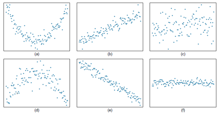
a) For which of these should you compute the correlation?

b) Among those for which it is appropriate to compute the correlation, which has a correlation closest to 1?

c) Among those for which it is appropriate to compute the correlation, which has a correlation closest to -1?

d) Among those for which it is appropriate to compute the correlation, which has a correlation closest to 0?

2. [OIS 7.4] Consider the following scatterplots:

 

a) For which of these should you compute the correlation?

b) Among those for which it is appropriate to compute the correlation, which has a correlation closest to 1?

c) Among those for which it is appropriate to compute the correlation, which has a correlation closest to -1?

e) Among those for which it is appropriate to compute the correlation, which have a negative correlation?

a) For each scatterplot, indicate whether or not it is appropriate to compute the correlation.

b) For those for which it was appropriate, which value of r listed above is the one most likely to be the correlation?

4. The scatterplots below each have a correlation listed among these numbers: r = -1, r = -0.85, r = 0, r = -0.48, r = 0.49, r = 1

a) For each scatterplot, indicate whether or not it is appropriate to compute the correlation.

b) For those for which it was appropriate, which value of r listed above is the one most likely to be the correlation?