
Regression Lines (short version)
In the previous section we converted the size and assessed values for the 14 houses we've been investigating:

to z-scores:
and noticed the shape and strength of the association remained unchanged. We then tried to find the "best-fit" line for this z-score scatterplot and found (using a bunch of basic yet tedious algebra) that in order for the line `hat(z_y) = m z_x + b` with m as slope and b as intercept to fit better than any other line, we needed b = 0 and
`m = (sum z_x z_y)/(n-1)`
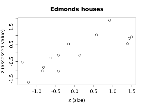
Using our house data, we computed that m = 0.81957, yielding an equation of `hat(z_y) = 0.81957 z_x` with a graph:

that fit the z-score data very well. The slope of (approximately) 0.82 told us that a house 1 size SD above the mean (zx = 1) is predicted to have an assessed value 0.82 assessed-value SDs above the mean.
Converting from z-scores back to the original units of square feet and thousands of dollars, we got the regression line for the house data (in the form `hat(y) = b_0 + b_1 x` where b0 is the intercept and b1 is the slope): `hat(y) = 249 + 0.038x`
We typically write this with more descriptive variable names: `hat(text(assess)) = 249 + 0.038 times text(size)`
If we graph this equation along with the original scatterplot of the house data, we get:
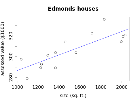
and we finally have our best-fit line for the house data. In practice, we won't use any of the formulas we've worked out to compute the slope and intercept of this line, we'll use technology instead. For now, let's concentrate on properly interpreting the linear equation once we've found it.
The slope of the regression line for the houses is 0.038. Remember that slope is "rise over run" (or "change in vertical (y) direction over change in horizontal (x) direction." The y-units for the house data are "thousands of dollars" and the x-units are (square feet), so the slope is:
0.038 `($1000)/(text(sq. ft.)`
which in simpler language is just: $38 per square foot. This tells us that each additional square foot in the size of the house is generally associated with an increase of $38 in the assessed value. This means that if a second house is $100 square feet bigger than the first, we would predict the second house to have an assessed value about $3,800 higher than the first. It does not mean that a second house will have an assessed value $3,800 greater than the first: in the scatterplot above, you can find pairs of houses where the bigger house is actually assessed at a lower value then the smaller house. And it does not mean that an increase in the size of a house causes an increase in assessed value: it may very well be the case that if you build an addition to your house, this will cause the county to assess it at a higher value; but it could also be that building practices have changed over time and the newer houses are bigger than the older houses, with the age influencing the assessed value, not the size.
The intercept of 249 might be interpreted as predicting an assessed value of $249,000 for a 0 sq. ft. house (in other words, a vacant lot) in this neighborhood. But we only have data about houses between 1,000 and 2,000 square feet in size, so making predictions about houses that are significantly larger or smaller (such as a vacant lot or a 6,000 sq. ft. mansion) involves extrapolation: this is dangerous because our model is based on information about houses of a certain size, and we don't know that the relationship between these variables continues to exhibit the same association for other types of houses.
Also keep in mind that our search for this regression line began with the assumption that the data had a linear association; if the data exhibits any sort of non-linear relationship (bending, curving, etc.) we should not attempt to find a regression line. (There may be other ways to model a non-linear association, but we'll save those for later.) To check that the data appears to have a linear association, we create a scatterplot, and we only create scatterplots when we have two quantitative variables, so we should only attempt to find a regression line when dealing with two quantitative variables. As we shall see soon, we also want to avoid using regression techniques when a data set contains one ore more significant outliers.
To summarize, before finding a regression line we should check that:
- we have two quantitative variables
- those variables exhibit a roughly linear (= non-curved) association
- a scatterplot of the data exhibits no significant outliers
Exercises
1. [OIS F7.6] The figure on the left (below) shows head length versus total length for 104 brushtail possums; the figure on the right shows weight city gas mileage vs. weight for a group of cars.
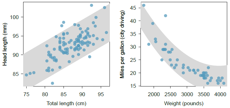
Answer the following questions for each data set:
a) Would a linear model be appropriate?
b) Would the slope of the regression line be positive or negative?
c) What units would the slope have?
2. [OIS F7.6] If we ask a computer to find a regression line to model the possum data shown in the previous problem, we get: `hat(y) = 41 + 0.59x`.
a) Rewrite this equation using more descriptive variable names.
b) If appropriate, predict the head length of a possum with total length of 92 cm.
c) If appropriate, predict the head length of a possum with total length of 62 cm.
d) If you observed two possums and the first had a total length 5 cm shorter than the second, what would predict about their head lengths?
e) Use a sentence to interpret the meaning of the slope in the regression equation.
f) Use a sentence to interpret the meaning of the intercept in the regression equation.