
Regression Lines (long version)
WARNING: Much algebra ahead. Don't spend time getting bogged down in the details on this page. Skim through if you need to, then skip to the next section, where we'll summarize the information from this page that you absolutely need to know.
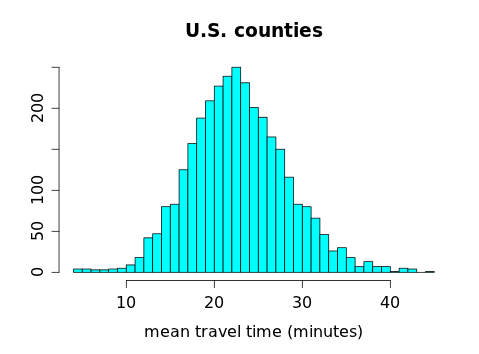
When we were learning to compute z-scores, we worked with a data set containing the mean commuting times (in minutes) for 3,143 U.S. counties during 2010, shown in this histogram:
We computed the z-scores for a handful of counties but if we were to convert every county's travel time to a z-score and make a histogram of all those z-scores, we'd get:
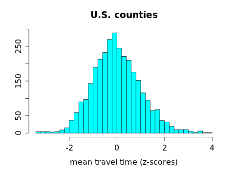
Notice that this looks almost exactly the same as the histogram for the actual travel times, because the z-score just shifts the data left (by subtracting the mean of all the travel times from each individual travel time) and scales the data in toward the center (by dividing by the SD of the travel times). The center and spread of the data change, but not the shape.
What is the center (mean) of the z-scores? It certainly appears to be 0, and in fact it is: the mean for the data set was 22.7 minutes, so when we subtract that value from the county in the exact center of the data set with a travel
time of 22.7 minutes, it gets shifted to 22.7−22.7 =0. So `bar z = (sum z)/n = 0` and this tells us that `sum z = 0` , the sum of all the z-scores in a data set, must be 0.
Now, the SD of the z-scores appears from the histogram like it might be 1, and it is, because we've scaled a time 1 SD above the mean to z = 1. The formula for SD is:
`sqrt((sum (z - bar z)^2)/(n-1))`
and since `bar z = 0`, it must be true that:
`sqrt((sum z^2)/(n-1)) =1 \ => \ (sum z^2)/(n-1) = 1 \ => \ sum z^2 = n-1`
so that tells us that if we square all the z-scores in a data set (for some reason) and add them up, we'll get 1. Keep this in the back of your mind.
z-scores and scatterplots
Now let's return to the scatterplot of size vs. assessed value for the 14 houses we've been investigating.

What if we converted all of the sizes to z-scores and all of the assessed value to z-scores? Well, we can certainly do that:
size assess z(size) z(assess)
1561 304.0 0.13 -0.13
1038 297.6 -1.38 -0.54
1224 289.5 -0.84 -1.05
1232 292.8 -0.82 -0.84
1995 314.6 1.39 0.53
1714 322.7 0.58 1.04
1832 336.1 0.92 1.89
1095 279.0 -1.22 -1.71
2011 319.5 1.43 0.84
1366 289.3 -0.43 -1.06
1292 301.4 -0.65 -0.30
1458 314.3 -0.17 0.51
2031 320.9 1.49 0.93
1366 304.0 -0.43 -0.13
mean 1515.4 306.12
SD 345.4 15.89
The first house, at 1561 square feet, has a size z-score of 0.13 (so it's 0.13 SDs above the average house size), and with an assessed value of $304,000, it has an assessed value z-score of -0.13, meaning it is 0.13 SDs below the average assessed value for these houses. In other words, it's a fairly typical house: just slightly above average in size and just slightly below average in assessed value.
For simplicity, let's call the size z-scores zx and the assessed value z-scores zy from now on. And let's graph zx vs. zy:
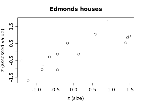
Compare this with the original scatterplot: the association looks exactly the same. The units have been scaled and shifted along each axis, but the relationships between the houses are unchanged. In particular, the strength of the association (the relative amount of scatter) appears to be exactly the same. (Keep that in mind for future reference, too.)
Now, let's try to find the "best" line that fits the z-score scatterplot. This line will have the form `hat(z_y) = m z_x + b` where m is the slope and b is the intercept. So the sum of the square of the residuals will be:
`sum (z_y - [mz_x + b])^2 = sum ([z_y - mz_x] - b)^2 = sum [(z_y - mz_x)^2 - 2b[z_y - mz_x] + b^2] = [sum(z_y-mz_x)^2] - 2b [sum z_y] +2bm [sum z_x] +[sum b^2]`
where we've use a bit of algebra. We know `sum z_y = 0` that and that `sum z_x` (remember those z-score facts from above) and the last term is just `b^2 + b^2 + cdots + b^2 = nb^2` .
So the sum of the squares of the residuals reduces to:
`[sum(z_y-mz_x)^2] + nb^2`
The first term is the sum of positive numbers (because they're all squared) and the second term depends only on n (the sample size, which is fixed) and b2, a positive number. To make this entire expression as small as possible, we need to have b = 0. So the intercept of the line in the z-score scatterplot is 0 and the equation for the line now looks like `hat(z_y) = mz_x`, and the sum of the squares of the residuals is:
`sum(z_y-mz_x)^2 = sum[z_y^2 - 2mz_x z_y + m^2 z_x^2] = sum[z_y^2] -2m[sum z_x z_y] + m^2 sum[z_x^2] = (n-1) - 2m [sum z_x z_y] +m^2(n-1) = (n-1)[m^2 -(2[sum z_x z_y])/(n-1) m +1]`
This last expression is (n-1), a fixed number, times a quadratic polynomial in m, which we can make as small as possible by finding the vertex of the associated parabola:
`m = -(B)/(2A) = -((-2[sum z_x z_y])/(n-1))/(2) = (sum z_x z_y)/(n-1)`
Whew! That's a lot of algebra. But it now tells us how to find the slope of the "best" line that fits the z-score scatterplot. We just have to multiply each zx by its corresponding zy, add those up, and divide by n−1.
size assess zx zy zxzy
1561 304.0 0.13 -0.13 -0.01763
1038 297.6 -1.38 -0.54 0.74075
1224 289.5 -0.84 -1.05 0.88188
1232 292.8 -0.82 -0.84 0.68739
1995 314.6 1.39 0.53 0.74055
1714 322.7 0.58 1.04 0.59970
1832 336.1 0.92 1.89 1.72861
1095 279.0 -1.22 -1.71 2.07610
2011 319.5 1.43 0.84 1.20752
1366 289.3 -0.43 -1.06 0.45751
1292 301.4 -0.65 -0.30 0.19204
1458 314.3 -0.17 0.51 -0.08542
2031 320.9 1.49 0.93 1.38771
1366 304.0 -0.43 -0.13 0.05770
Adding up all of the products in that last column, we get 10.65441, and finally we divide that by 13 to get: 0.81957
So the equation of the line is `hat(z_y) = 0.81957 z_x` and when we graph that with the z-score data we get:

which looks like it's better than any other line we could draw. Notice that because the intercept is 0, this line passes through the point where zx = 0 and zy = 0, which represents a house of average size and average assessed value. The slope of (approximately) 0.82 tells us that a house 1 size SD above the mean (zx = 1) is predicted to have an assessed value 0.82 assessed-value SDs above the mean.
But we don't usually deal in z-scores when discussing real estate, so we need to convert this equation back into our regular units. We recall the z-score formula and write:
`(hat(y)-bar(y))/(s_y) = 0.82 ((x-bar(x))/(s_x)) => (hat(y)-306.12)/(15.89) = 0.82((x-1515.4)/(345.4)) => hat(y) = 0.82((15.89)/(345.4))(x-1515.4) + 306.12 => hat(y) = 0.038x+249`
In statistics, we usually write this line, which we call the regression line for the given data set, in the form `hat(y) = b_0 + b_1 x` where b0 is the intercept and b1 is the slope.