
Linear Models
We've recently used the Normal distribution as a mathematical model for certain unimodal, symmetric quantitative variables. We now investigate a model for certain relationships between two quantitative variables.
Property taxes
Recall the data about the single-family residences on a street in Edmonds, Washington, that we examined when first constructing a scatterplot. The data set includes 14 cases (each house is a case), and the variables are: house number, the size (in square feet), the 2007 assessed value (in thousands of dollars), the lot size (in acres), the 2006 taxes (in dollars) and the number of stories. Here is the complete data set for reference:
| house | size | assess | lot | taxes | stories |
| 20911 | 1561 | 304 | 0.2 | 2604 | 1 |
| 20912 | 1038 | 297.6 | 0.2 | 280 | 1 |
| 20918 | 1224 | 289.5 | 0.17 | 2353 | 1 |
| 20921 | 1232 | 292.8 | 0.17 | 756 | 1 |
| 20924 | 1995 | 314.6 | 0.17 | 2620 | 2 |
| 20927 | 1714 | 322.7 | 0.18 | 2632 | 1 |
| 20930 | 1832 | 336.1 | 0.18 | 2779 | 2 |
| 21003 | 1095 | 279 | 0.18 | 2321 | 1 |
| 21006 | 2011 | 319.5 | 0.18 | 2663 | 2 |
| 21015 | 1366 | 289.3 | 0.18 | 2415 | 1 |
| 21018 | 1292 | 301.4 | 0.18 | 2477 | 1 |
| 21023 | 1458 | 314.3 | 0.18 | 1386 | 1 |
| 21028 | 2031 | 320.9 | 0.18 | 2676 | 2 |
| 21105 | 1366 | 304 | 0.18 | 2473 | 1 |
and here is scatterplot of size (which we treat as the explanatory variable) vs. assessed value (the response variable):

We characterize the association apparent in this scatterplot as positive, linear and moderately strong, with no obvious outliers. Because this data generally follows a linear pattern, let's see if we can draw a line that follows this pattern somewhat closely:
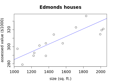
If we had every student in the class draw such a line, it's likely that none of them would look exactly like the blue line above (or each other), but most of them would be reasonably close. Can we determine which of these lines is "best" (or at least better than the others)? The blue line doesn't pass through many of the points (it may not exactly pass through any of them) but it comes close to quite a few. We first need to decide how we're going to measure this "closeness."
To do so, let's think about how we might use the equation for this line if we could find it. One use would be if we had a similar house of known size (say, 1400 sq. ft.) on a similar nearby street about which we wanted to estimate its assessed value. The blue line above has equation y = 0.045x + 240, so we could plug in 1400 for x and the resulting y-value, y = 0.045(1400)+240 = 303, so we would estimate this house's assessed value at $303,000. Now, this estimate might be close to the actual assessed value of the house, or it might not, but the accuracy of the estimate could then be measured by the difference between the actual value and estimated, or predicted, value. We call this difference a residual:
residual = actual − predicted
In alternative notation, we sometimes write:
`e = y - hat y`
where e stands for the residual, y is the actual y-value of a particular house and `hat y` is predicted value we get from using the equation of the line, which we now write: `hat y = 0.045x + 240`
Since the 1400–square-foot house was imaginary, we can't check the estimated value against the predicted value, but we could compute the residuals for the 14 houses in the original data set:
size assess predicted residual
1561 304.0 310.245 -6.245
1038 297.6 286.71 10.89
1224 289.5 295.08 -5.58
1232 292.8 295.44 -2.64
1995 314.6 329.775 -15.175
1714 322.7 317.13 5.57
1832 336.1 322.44 13.66
1095 279.0 289.275 -10.275
2011 319.5 330.495 -10.995
1366 289.3 301.47 -12.17
1292 301.4 298.14 3.26
1458 314.3 305.61 8.69
2031 320.9 331.395 -10.495
1366 304.0 301.47 2.53
First we compute the predicted value for each house: for the first one we get 0.045(1561)+240 = 310.245. Then we compute the residual: for the first one we get 304.0−310.245 = -6.245. (Check the computations for a couple of the other houses in the above table to see how this works.) Some of these residuals are negative (meaning that the predicted value was too high) and some are positive (meaning that the prediction was too low).
In order to make accurate predictions with our linear model, we'd like the residuals—which are the "errors" in the predictions for the given data values (this is why we use e as our notation for a residual)—to all be as close to 0 as possible. Another way to think of this is that we want the residuals to vary as little as possible from 0. How have we measured variability before? With a standard deviation. And how did we compute that? We computed the deviations from the mean, squared them, added them up, divided by n−1, and took a square root. We could do something like that here with the deviations between the residuals and 0:
`sqrt((sum (e-0)^2)/(n-1)) = sqrt((sum e^2)/(n-1))`
We want to make this "total deviation" as small as possible, but it will attain a minimum exactly when the expression inside the square root attains a minimum. (You may have solved story problems in other math classes where you minimized the square of a distance when you really wanted to minimize a distance, because it was easier to do the math without the square root in place; the same principle applies here.) So we want to make this:
`(sum e^2)/(n-1)`
as small as possible. But of course the denominator of that fraction is fixed (for example, if we start with 14 houses, the denominator will always be 13), so the only way to make the fraction as small as possible is to make the numerator as small as possible. This means that what we really want to do is to minimize the sum of the squares of the residuals:
`sum e^2`
For the blue line above, if we compute squared residuals:
size assess predicted residual residual^2
1561 304.0 310.245 -6.245 39.000025
1038 297.6 286.71 10.89 118.5921
1224 289.5 295.08 -5.58 31.1364
1232 292.8 295.44 -2.64 6.9696
1995 314.6 329.775 -15.175 230.280625
1714 322.7 317.13 5.57 31.0249
1832 336.1 322.44 13.66 186.5956
1095 279 2 89.275 -10.275 105.575625
2011 319.5 330.495 -10.995 120.890025
1366 289.3 301.47 -12.17 148.1089
1292 301.4 298.14 3.26 10.6276
1458 314.3 305.61 8.69 75.5161
2031 320.9 331.395 -10.495 110.145025
1366 304.0 301.47 2.53 6.4009
and add them up, we get 1220.863. Of course, that doesn't mean much unless we have something to compare it to. If we try this whole process with a different line, say `hat y = 0.03x + 250` (shown in red):
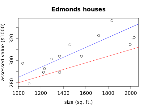
we can compute the sum of the squares of the residuals to be 2762.413. This tells us that blue line is better than the red line (which is more or less obvious from the graph), but the question remains: can we think of another line that would be better than the blue line?
The answer is yes, but to find it, we'll need to take a slight detour.
Exercises
1. Show that the sum of the squares of the residuals for the red line is 2762.413.
2. Guess another slope and intercept that might work better than the blue line. Test it by computing the sums of the squares of the residuals.
3. In the equation y = 0.045x + 240 (shown in blue in the graphs above):
a) What is the slope of the line?
b) What would the units of that slope be?
c) What might the slope mean in relation to the sizes and assessed values of these houses?
d) What is the y-intercept of this line?
e) What would the units for the y-intercept be?
f) Where does the blue line cross the vertical axis in the scatterplots shown above?
g) Why doesn't it cross at the y-intercept?
h) What meaning might the y-intercept have in relation to the sizes and assessed values of these houses?